Collaborative Filtering: how our network influences the movies we watch and products we buy
In part three of our series on recommendation systems, we're talking about harnessing the preferences of a network of users through collaborative filtering.
Welcome to the third post in a series about recommendation systems. In the first two posts, we talked through the basics, examples, and dove into what makes a content-based recommendation system. Start here to catch up on the series, then go here for the second post.
the downfall of content-based recommendation systems
Recap: Last week, we talked about content based recommendation systems and how they use a user’s past feedback, both implicit and explicit, as well as attributes about the items that are being recommended as inputs. The distance between a vector representation of both the user and the attributes is then measured and the similarity metric output is then used to yield a prediction.
But there’s something missing from this equation. What about all the other users on a given platform? And their preferences, feedback, likes and dislikes? If we were to utilize their data too, we’d could paint a more holistic picture of what to recommend within the system.
collaborative filtering
Introducing, collaborative filtering - the second recommendation system we’ll be walking through in this series.
What’s collaborative filtering? A type of recommendation system that utilizes similarities in preferences among a larger network of users to produce recommendations in the style of “Similar users liked…”.
If you think about it from the phrase itself —
collaborative emphasizes using the preferences of other users to pick better recommendations for a given user
filtering emphasizes deciding which items fit best with a given set of user preferences (that could be thought of like filters)
There’s two main types — item-item and user-user. Item-item typically outperforms user-user in practice due to the varied taste of users and how meaningful item-item similarities are.
User-user focuses on patterns between similar users, assuming that users with similar preferences in the past will most likely have similar preferences in the future.
Item-item focuses on similarities between items, assuming that items that are similar are likely to be preferred by similar users.
how it works
To build a collaborative filtering model from the user-user approach, we need users, items, and their preferences/feedback about those items. Not all users need to have given feedback to all items - matter of fact the places that users haven’t given feedback is where we will work to predict what their feedback would be.
As a preface, collaborative filtering gets pretty mathy pretty quickly. I’m going to do my best to give an explanation at a high level, share the terms you need to know, and let you know where to find resources if you want to dig deeper.
the user-item matrix
Last week, we talked about one user and many items. Mathematically, we really only had a single user vector and multiple items vectors. In collaborative filtering, we take a different approach. What if we had multiple items and multiple users with their preferences represented in a matrix?
Using content-based recommendation systems, we showed how to build the “Top Picks for Gaby” feature from Netflix. This week, using collaborative filtering, we’re going to build a system that shows recommendations based on what “users like you watched”.
Using a dataset like MovieLens, we will aggregate our users’ preferences. We can use either implicit or explicit feedback to represent a user’s preferences.
Implicit feedback is behaviors of a user that demonstrate preference such as clicking on an item or viewing an item (like watching a movie).
Explicit feedback is a rating or review of an item in the system given by the user.
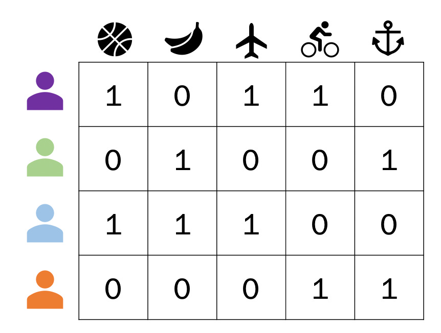
For our example1, we’re going to use the implicit feedback of a user watching a movie as a boolean — either 0 because they haven’t watched or 1 because they have watched — representation of preference. If we gather all movies our users have watched, we can generate a matrix representation of which movies they’ve watched and haven’t, like the user-item matrix below.
We have 4 users and data on whether they have or haven’t watched 5 movies. We want to supplement this data with information on each of our movies. This brings us to embeddings.
what is an embedding?
Depending on the context, “embedding” can mean different things. In machine learning, embeddings are a lower dimensional space that numerically represents complex, multi-dimensional, and not always machine readable information. Sound complicated? It’s easier to digest when we use an example.
We need to supplement our model with information on the movies themselves. Let’s create a line, with possible values from -1 to 1 along it representing the range of movie types from drama to comedy. On this line, let’s plot where our users’ preferences lie as well as where a given movie falls.
How to interpret: Purple person really likes dramas, and we’ll represent that with a scalar value of -1. The plane movie is a drama with a touch of comedy, so we’ll give it a value of -0.5. We are hand building embeddings to represent preference and movie type respective to dramas versus comedies.
A good note from the folks at Google — “We represented both items and users in the same embedding space. This may seem surprising. After all, users and items are two different entities. However, you can think of the embedding space as an abstract representation common to both items and users, in which we can measure similarity or relevance using a similarity metric.”
We can repeat this process with several other variables, like movie content rating (kids to R), age of the movie (old to new), and more. We’ll get numeric representations of how our users are interested as well as how our movies rank on the spectrum of [-1, 1] and these are our embeddings.
Our system is now even more powerful. We have scalar values that represent where our movies fall on a spectrum of variables, as well as scalar values that represent our users’ preferences on these variables. These values will inform the next step of the process — matrix factorization.
matrix factorization
Remember how I said things get pretty mathy, pretty quickly? We’ll keep things light, but buckle up.
We have vectors made up of scalar values that represent both our user’s preferences and the details of our movies. Matrix factorization is a process that’s been a mainstream method to generate collaborative-filtering recommendations since Simon Funk, part of the third place team on the Netflix Prize, released his work on the topic in a blog post in 2006.
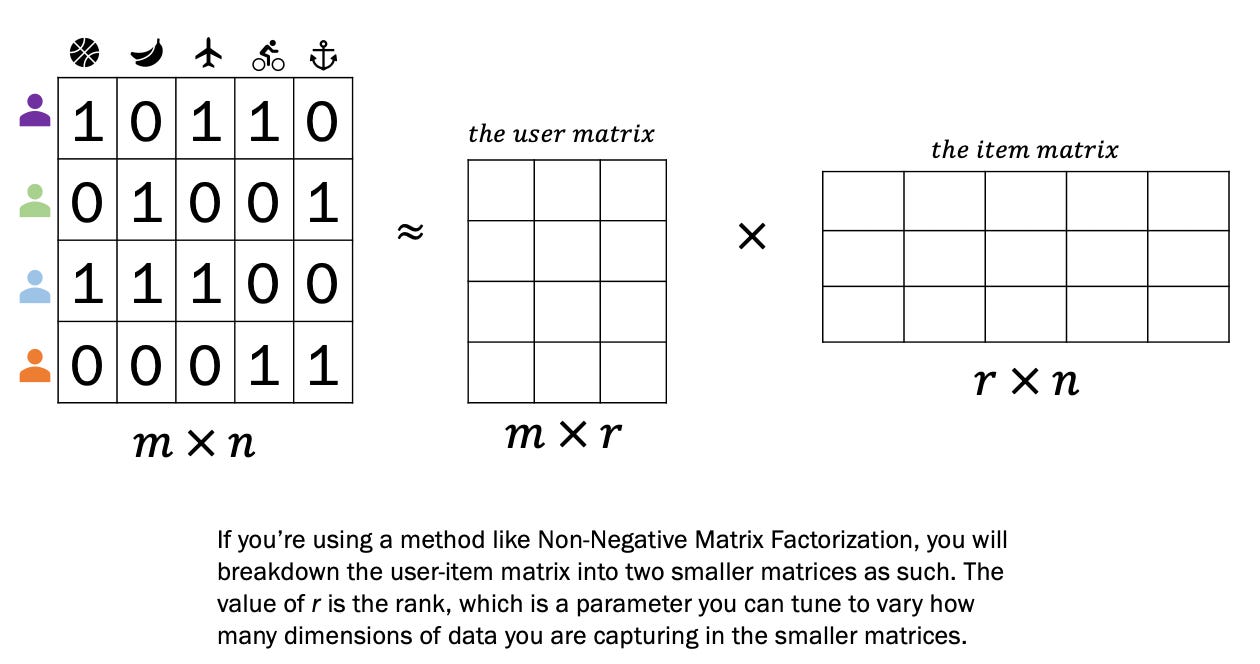
High level, matrix factorization takes our user-item matrix and breaks it down into a user matrix and an item matrix. It’s from these smaller matrices that we are able to generate predictions.
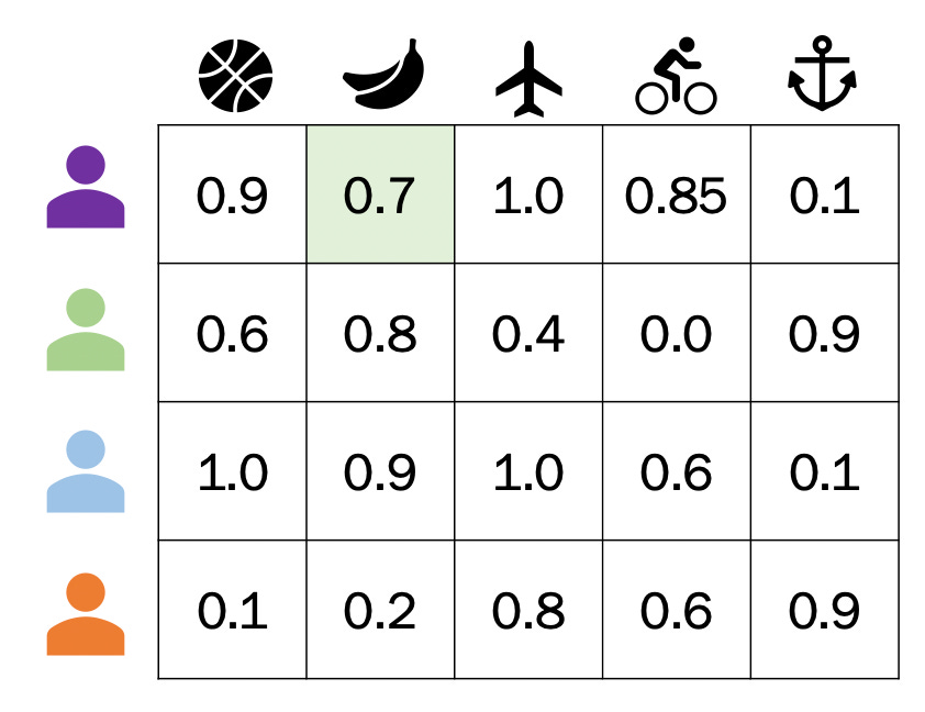
See how, in the visual above, the two matrices when multiplied are approximately the user-item matrix (the squiggly equals sign means approximately)? Through matrix factorization, we’re able to get approximate values for what a user thinks about a movie they haven’t watched. If we were to multiple the resulting two matrices, we’d get a 4 by 5 matrix of predicted values that’s an approximate representation of the user-item matrix. It could look something like this:
The values that are closer to 1 for a user means the model believes that user would watch that movie. By filtering out movies they’ve already watched, we can make our recommendations. For our Purple user, it looks like we should recommend them the Banana movie! They’ve never seen it, but based on the data we’ve gathered on other users and the type of movie it is, we think they’d like it.
Took us some math but we made it!
in the real world
We built up embeddings by hand, identifying relationships and attributes of our data. In a true collaborative filtering model, these relationships are learned through the development and training of models. Algorithms can learn these relationships and figure out ways to extrapolate similarities between users and items to complete this process at scale. There’s also much more data to be used in a real recommendation system which can grow matrices to millions of rows with millions of dimensions of data.
the downside of collaborative filtering
It’s called the “Cold Start” problem. You need users in the system that have given ratings to really harness the power of collaborative filtering. You also can’t recommend items that haven’t received feedback yet. These issue tend to be downsides of collaborative filtering that content-based filtering can help address. Using these methods together can lead to powerful predictions, no matter how long an item or a user has been in the system.
where to learn more
This 20 minute Stanford lecture on collaborative filtering and this lecture on how to implement
Google Developer course — a great, basic overview, that inspired much of this article
Recommender Systems: The Textbook — some sections and corresponding materials can be found online
Simon’s blog post on Matrix Factorization
Methods Used for Matrix Factorization
Surprise — a Python library for recommendation systems
that’s a wrap
Thanks for reading another week of Day to Data! We’re wrapping up our recommendation system series next week, then will pivot back to regular programming after that. As always, if you have any thoughts, feedback, or ideas for what to cover next, let me know!
Example modified from Google’s Developer course on Collaborative Filtering


