If a decision tree falls in the forest

The basics of decision trees - classification, regression, and random forests

Today, we’re talking about decision trees. As one of the most foundational elements of data science still widely used today, decision trees walked so modern day machine learning could run (more like sprint full speed ahead). We’re going to get down to basics and not overcomplicate things. Let’s talk decision trees.

Modeling human behavior

If you dive into the rabbit holes of the history of data science, you’ll find a fascinating pattern — several prominent data science techniques stem from human behavioral or psych studies. We’ve talked about one already — the reinforcement learning that now makes GPT-4 so powerful has its roots in behavioral studies about reward and punishment originally completed on rats!

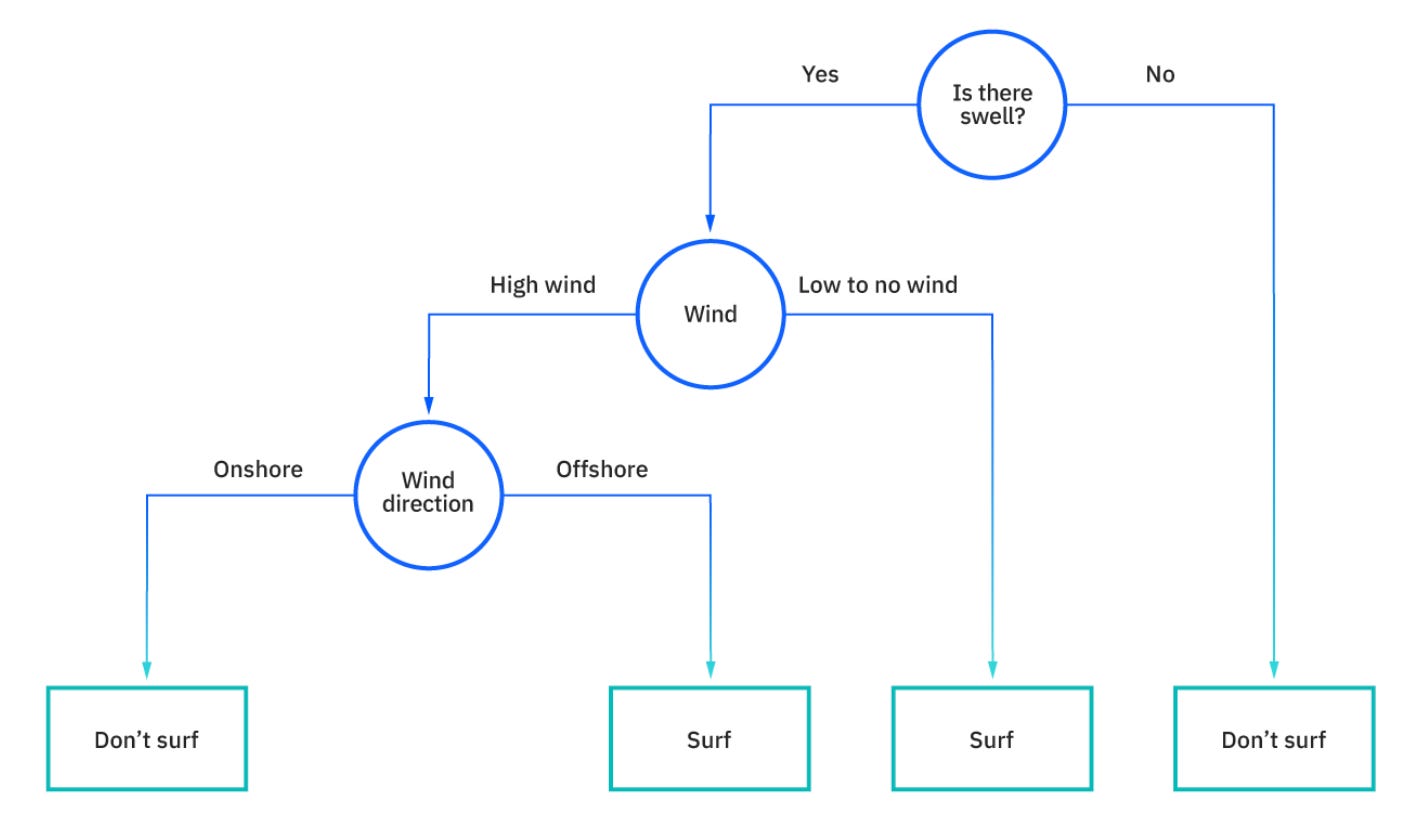
Decision trees also have roots in human behavior. While the exact history of the decision tree is quite ambiguous, decision trees are something humans do at an incredibly fast speed, hundreds if not thousand of times a day. Before I want to go surfing, the chart below is a pretty good representation of the inner monologue I’ll conduct to result at a decision of “surf” or “don’t surf”. The technical process of decision trees mirror much of this inner dialogue.

Source: IBM

All about the fundamentals

Decision trees do two things really well — classification and regression. Classification is simple — surf or don’t surf. Regression can be a bit harder to visualize. Instead of predicting a class (surf or don’t surf), the decision tree algorithm is trying to predict a numeric output, like price or temperature. Each method is used for a different purpose, and the accuracy of the algorithm differs in how its measured depending on if you’re solving a classification or regression problem.

Classification

To surf or not to surf! As we saw in the graph above, imagine a dataset where each entry represents a day, and the features in the dataset include information around the swell, wind speeds, wind direction, and more. With the historical data and classification decision tree, you can begin to train a model on the thresholds that may result in surfing or not surfing. For example, if the wind is less than 10MPH, the swell is between 1-3 feet, and the wind direction is in the offshore direction, go surf! But if the wind is greater than 30MPH regardless of any other data point, don’t go surfing. Classification models use thresholds on numeric inputs as decision points to get closer and closer to a final decision. The performance of a classification decision tree can be measured using a metric called F1 (unrelated to the driving) that represents the precision and recall of the model. Sometimes it’s ok to ignore the data though and just go surfing for the fun of it :)

Regression

How much is that house worth? A decision tree solving a regression problem like this will evaluate how much each feature in a dataset plays into the target variable. We may have a dataset with features like number of bedrooms, square footage, or price per foot average in the county that feed into the final value of the home. A regression model can take these inputs (features) and learn a set of decisions that will predict the price of a given home. This model, once trained on historic home values, can predict values for homes in the future on data it hasn’t seen before, resulting in a numeric prediction. The performance of a regression model is measured by seeing how far away a prediction is from the actual value, by using a metric like mean squared error.

Downfalls of decision trees

Not everything is perfect!

1. Overfitting: Let’s use dogs as an example. So you have a dataset with 100 dogs and their breeds. You’re trying to predict what breed a given dog is based on a photo. Overfitting would be if your model simply memorized the 100 dogs and their breeds in it, but the 101st dog you showed the model would be very hard for it to predict what it was. It didn’t generalize well.

   Ideally your model would start to pick up on patterns - golden retrievers and yellow labs are about the same size, a mastiff and Saint Bernard are both big dogs, or that Dalmatians and Great Dane’s can both have spots — rather than “hard-code” the definitions from your training dataset.

2. Imbalanced datasets: So you have a dataset that includes credit card transactions, labeled as “fraudulent” or “not fraudulent”. 98% of the transactions are not fraudulent. Only 2% are not fraudulent. Decision trees tend to struggle in this situation - they’re bad at predicting minority classes in imbalanced datasets (fraudulent transactions in this case). If you built a model for this dataset and just predicted “not fraudulent” for every transaction in that dataset, you’d be accurate 98% of the time! What good is that? You’d be 100% wrong at finding the 2% that are fraudulent. Imbalanced datasets require extra care and understanding for data teams to build robust, valuable models.

What comes after decision trees?

Decision trees include simple logic, but they do have their disadvantages. One tree can be useful, but what if there was a forest!? That can be really powerful!

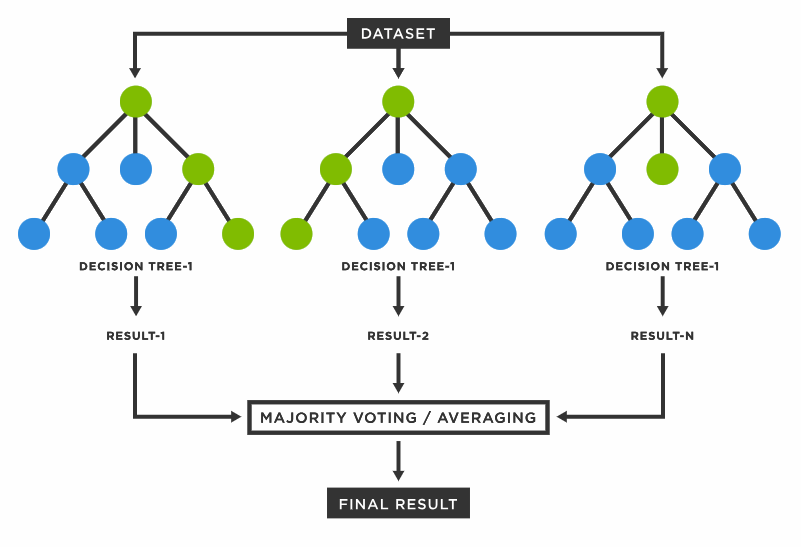
Random forests utilize multiple decision trees to get to a single result. It can handle regression and classification, while providing better accuracy and flexibility. Random forests came after the bagging technique was established in 1996 by Leo Breiman. Bagging is a method where you can select a sample of data points from a dataset with replacement (meaning one data point can be chosen multiple times) and build several models. The average or majority of predictions from each model get you to a more accurate prediction than one decision tree model alone. Bagging can use other types of models, not just decision trees. Random forests, however, are an extension of the bagging technique with decision trees, with elements of randomness! Instead of using all the features in a model, random forests select subsets of features at random to ensure no dependence on a single variable is too strong, resulting in poor model performance. We could talk for a while about the intricacies of random forests, but instead, here’s a good article if you want to get into the details.

Source: TIBCO.

---

Thanks for reading this week’s Day to Data! Next week, we’ll be talking about a buzzword that’s recently joined my regular vocabulary now that I’m an investor — data moats. More data in the future. Stay tuned!